Model Merging and the Geometry of Optimization

22 Dec, 2025

TL;DR: Here I’m revisiting older notes on model merging. Gradient descent steps can be viewed as model merges, and model merges can often be interpreted as gradient steps. Making this connection explicit shows that smooth merging methods recover pre-conditioned gradient descent, while linear merging implicitly assumes a Euclidean geometry. When models are trained with different optimizers or pre-conditioners, this assumption can fail, helping explain when naive averaging works and when geometry-aware merging methods are needed.

Gradient steps as model merging

Consider a model ${\theta }_0$ that we wish to optimize with respect to a loss $L$ over a dataset $B$. We will use batch gradient descent (GD) to carry out the optimization, here's the first step of this given some $\eta >0$:

We can massage this equation to get

Thus we wrote the GD step as a linear-model-merge (often called LERP) between the original model ${\theta }_0$ and a unit-step local model ${\theta }_L:=({\theta }_0-\nabla L_B({\theta }_0))$ (“local” to the dataset/batch we use, which is different from the local models from federated learning¹). We expect that ${\theta }_L$ has a smaller loss than ${\theta }_0$².

Local-model substitution: Using ${\theta }_A:=\theta$ and ${\theta }_B:=\theta -\nabla L_B(\theta )$ (or ${\theta }_B(\eta ):=\theta -\eta \nabla L_B(\theta )$) as the models in a merging method.

It’s reasonable to try to work backwards from a model merging method to recover an optimization method by using the local-model substitution discussed here to see what optimization methods pop out. For example,

• In the single-task case, TIES³ reduces to sparsified (top-k) gradient descent.
• For small $\eta$, a SLERP-merge of ${\theta }_A$ and ${\theta }_B(\eta )$ is behaving like regular gradient descent.

For smooth model-merging methods, the ${\theta }_A,{\theta }_B$ substitution never gives surprising results, in some sense:

Lemma 1 (Smooth merging functions recover GD steps with small step-size)

Let $f:{ℝ}^n\times {ℝ}^n\to {ℝ}^n$ be a $C^1$ “merging” function, mapping $({\theta }_a,{\theta }_b)\mapsto {\theta }^{\prime }$, and assume:

1. Consistency: for all $\theta$, $f(\theta ,\theta )=\theta .$

2. Jacobian at the diagonal: the partial derivative w.r.t. the second argument exists and

   ${\frac{\partial f}{\partial {\theta }_b}|}_{{\theta }_b=\theta }=A$

   for some matrix $A$.

Define the update

Then, as $\eta \to 0$,

So a smooth merging function recovers a pre-conditioned GD method in the small $\eta$ limit.

Proof

Since $f$ is $C^1$, we can Taylor expand in the second argument around $\eta =0$ (i.e., around ${\theta }_b={\theta }_n$):

Using the assumptions $f({\theta }_n,{\theta }_n)={\theta }_n$ and ${\frac{\partial f}{\partial {\theta }_b}|}_{{\theta }_b={\theta }_n}=A$, we obtain

which concludes the proof. $◻$

When $\eta \approx 0$, we have ${\theta }_n\approx {\theta }_n-\eta \nabla L({\theta }_n)$, so the two “models” being merged are extremely close in parameter space. This regime is not representative of most practical model merging settings, where models are typically separated by many optimization steps.

Next we look at the opposite direction: from model merging to gradient steps.

Linear model merging as gradient steps

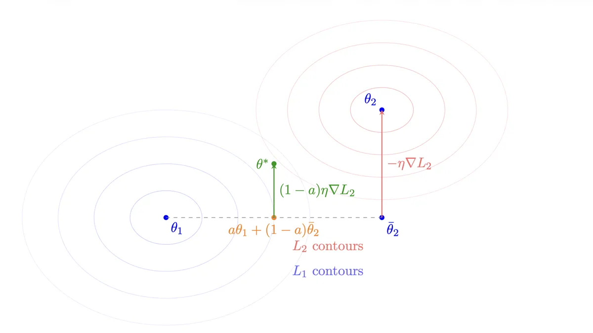
Consider two models ${\theta }_1$ and ${\theta }_2$ derived from a common initialization ${\theta }_0$ and optimized on different loss functions $L_1$ and $L_2$ respectively using gradient descent. Therefore, we get that, for ${\theta }_2$, there exists a point ${\overline{\theta }}_2$ and learning rate $\eta$ such that:

Those⁴ have to exist as they represent the last optimization step that resulted in ${\theta }_2$.

Now, for a linear model-merge with interpolation parameter $a\in [0,1]$:

By substituting the gradient descent representation of ${\theta }_2$:

Thus the merged model ${\theta }^{*}$ can be seen as a gradient descent step where:

• The starting point is the weighted average $a{\theta }_1+(1-a){\overline{\theta }}_2$
• The step is in the direction of $\nabla L_2({\overline{\theta }}_2)$
• The effective learning rate is $(1-a)\eta$

So linear model merging is taking a partial gradient step from an interpolated position in parameter space, with the size of the step modulated by the merge coefficient $a$.

Riemannian geometry and model merging

Lemma 1 says that smooth model merging methods, when used with the local-model substitution we discussed earlier, behave like pre-conditioned gradient descent. In light of all this, I think we can sense-check linear model merging when used with models that optimize under different optimizers.

Suppose we have ${\theta }^{(1)},{\theta }^{(2)}$ representing the model parameters of two models trained with the losses $L_1,L_2$ and different optimization schemes, which we will assume are:

where $k=1,2$ and $P_k$ are pre-conditioners, $P_1\ne P_2$, symmetric and positive-definite, ${\eta }_k>0$, and we assume those are converging to ${\theta }_{*}^{(1)}$ and ${\theta }_{*}^{(2)}$.

Without getting too deeply into Riemannian geometry, the existence of pre-conditioner $P_k$ in gradient descent (GD) means that each corresponding GD makes steps in a geometry with metric $G_k=P_k^{-1}$. We can then measure the distance of a $\theta$ from ${\theta }_{*}^{(k)}$ by using

which uses the metric that each GD is optimizing in. For example, if $G_k=\mathrm{d}\mathrm{i}\mathrm{a}\mathrm{g}(1,100)$, the corresponding $J_k$ would penalize harshly deviations in the second dimension.

Given this, we would want a successful merge to be close to

It turns out that we can find ${\theta }_{\mathrm{o}\mathrm{p}\mathrm{t}}$ exactly as everything is linear:

Toy example

Now, we assume $G_1=\mathrm{d}\mathrm{i}\mathrm{a}\mathrm{g}(100,1)$ and $G_2=\mathrm{d}\mathrm{i}\mathrm{a}\mathrm{g}(1,100)$, ${\theta }_{*}^{(1)}=(0,0)$ and ${\theta }_{*}^{(2)}=(1,1)$.

• Linear merge: ${\theta }_{\mathrm{l}\mathrm{i}\mathrm{n}}=0.5{\theta }_{*}^{(1)}+0.5{\theta }_{*}^{(2)}=(0.5,0.5)$
• Optimal merge: ${\theta }_{\mathrm{o}\mathrm{p}\mathrm{t}}\approx (0.0099,0.9901).$

We can also compute the errors according to $J_{\mathrm{m}\mathrm{e}\mathrm{r}\mathrm{g}\mathrm{e}}$.

and

As expected, the optimal merge has much smaller error compared to the naive merge because the naive merge does not account for the geometry.

This toy example illustrates a general failure mode of naive linear merging. When models are trained with different pre-conditioners (or even different optimizers!), they implicitly optimize under different geometries. Linear interpolation assumes a shared Euclidean geometry and therefore computes the wrong midpoint. The resulting merged model can be arbitrarily far from optimal⁵.

Notably, several existing merging methods can be understood precisely as attempts to respect this geometry, e.g., Fisher merging⁶, Ties-merging, etc.

Footnotes