Local theory for neural thickets
Cross-posted this to alphaxiv.
I read the Gan, Isola 2026 paper on neural thickets. If we start from a pre-trained model, we can use fine-tuning to convert the model into a task-expert, e.g., a model better at math questions, by following gradients w.r.t some training set. What Gan and Isola claimed is that some large models have some of those task experts relatively close in the weight space -- close enough that they can be reached through random search!
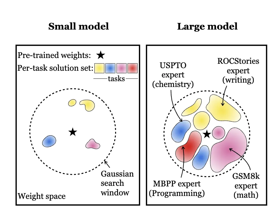 Image is from the Gan, Isola paper.
What is of interest here:
- Large models that have been pre-trained on a lot of tasks can develop thickets: neighborhoods in the weight space where tasks experts are reachable with random perturbations of the base parameters.
- We can validate the performance of the perturbed models with some task-specific validation set and keep the best K out of N.
In this post, I wanted to explore how a local theory of thickets would look like and how much it would predict:
- How far should we look for the best perturbations?
- What is the best performance we can expect from the top expert?
What we show is that in the local regime, we can predict the answers by using the per-task gradient and Hessian. On six small LLMs, this prediction holds for small , although the gains are small.
Local improvement theory
We will denote the parameters of a model by .
We have tasks, defined in terms of losses , where where positive semi-definite and symmetric and is a minimum of . Next, we also define the combined loss
At , . This is not zero at except if . Typically represents a compromise between tasks, so this is expected.
Perturbations: we assume , where and
What we are interested in is the difference in loss if we use instead of for task :
or we may talk about the "improvement", i.e.,
The average perturbation hurts: (here we used ).
Best-of-N improvement
The idea is that we sample and we want to pick the best perturbations with respect to . This corresponds to tracking what the best expert can do.
Inner product with MV IID Gaussian gives univariate Gaussian: and is a constant vector,
Trace approximation: . Assuming is large enough and the columns of are spread out enough, a plausible approximation is
Using the trace approximation decouples the second term from ! We can write the improvement as:
To get the best improvement, we sample and pick the one that gives the best improvement, i.e., the largest negative in the sample. We can ballpark that as to get:
This also allows us to solve for the best :
which finally gives the best improvement:
As a reminder, is the number of samples we get from , and is the Hessian at . In practice, we can estimate by using an estimator of .
Experiments
The best-of- improvement depends on the model only through two numbers, and . Those don't depend on the perturbations.
Setup.
- Models: six small instruct models: Qwen2.5 at 0.5B, 1.5B, 3B and 7B, LFM2-1.2B and SmolLM2-1.7B.
- Task: GSM8K. The loss is the per-token negative log-likelihood of the reference solution, averaged over 64 problems. That's the equivalent of the selection set from the Gan and Isola paper.
- Measuring the two numbers: comes from one backward pass. comes from a Hutchinson estimate, the average of over 20 random sign1 vectors .
- Sampling: at a few values of around the predicted , I sample 100 directions and evaluate both and . That gives perturbations and keep the best improvement.
The plot. The six models differ a lot:
- ranges from 4 to 42.
- ranges from to .
- ranges2 from to about .
To compare them on one plot, we can rescale each point.
- On the -axis is .
- On the -axis is the measured gain divided by the predicted best gain. In these units, the prediction for every model is the same parabola:
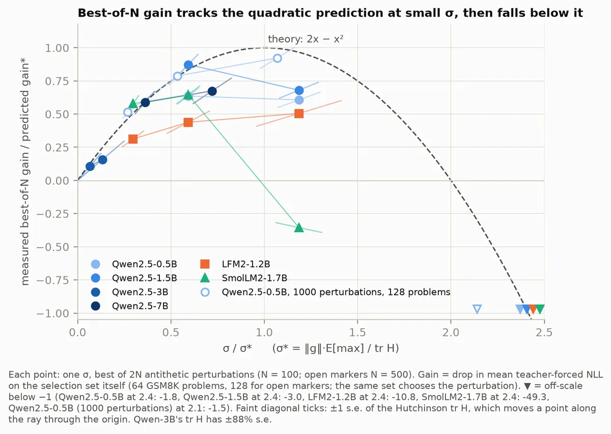
For , we see close agreement with the curve. This includes models whose differ by more than a factor of 10, so it's not one lucky fit. Beyond that we lose agreement as higher order terms start to matter more.
To be clear, the gains are small. The best perturbation raises the probability the model gives to each correct token by about 2% (Qwen2.5-0.5B), and by up to about 10% for the other models.
Does it carry over to new problems? For Qwen2.5-0.5B I repeated the experiment with 128 selection problems and 128 fresh held-out problems. The perturbation that won on the selection set keeps 84–92% of its improvement on the held-out set. The reason is that the gradients of the two sets point almost the same way: .
What about accuracy? The loss here is NLL. As it is smooth, it is expected that for small enough local theory applies well. Measuring accuracy under each perturbation means generating fresh answers from every perturbed model. I didn't do this with LLMs due to cost + noise, but on a toy problem accuracy was also predicted.
Caveats.
- These are small models and a single task.
- The 3B model's estimate is noisy.
- The 64-problem plot is a selection-set result. The held-out check uses only one model.
- The plot uses the exact expected maximum of 200 standard normals, , rather than the ballpark from the derivation above. The ballpark overestimates the best gain.
Related Work
Neural Thickets
Gan and Isola's paper got a fair amount of follow-up. The two I found most useful:
- Dufour et al. show you don't need to touch the weights at all: adding a random bias to the output logits works about as well on most reasoning tasks. Their take is that the gains come from diverse outputs, selection and voting.
- Asilis et al. argue that most of the "expert" lift is selection noise. Pick the best of many noisy scores and it will look good on the selection set, much less so on held-out data.
Evolution strategies
The local theory in this post is not new. The expected improvement from picking the best of random perturbations on a quadratic was worked out in the evolution strategies literature, most generally by Akimoto, Auger & Hansen, building on Beyer's The Theory of Evolution Strategies (2001). What I add is measuring the two things that theory needs, the gradient norm and the Hessian trace, on actual LLMs.
For ES on LLMs, see Qiu et al. and Liang et al.. Liang et al. argue that the curvature of LLM fine-tuning landscapes lives in a few directions, which is why small ES populations work.