Lifting gradient flows

05 May, 2026

In the previous post we talked about creating attracting manifolds and how to get the corresponding vector field given a manifold. In this one, we talk about optimization.

Suppose we have $g : ℝ \to ℝ$ for which we want to find a minimum and $g$ is sufficiently smooth. For example, we can consider

def g(x): return 0.25 * (x * x - 1.0) ** 2 + 0.18 * x

That's a simple function with two minima, one local and one global. If we use the gradient of $g$ , we can create a vector field on the curve by pointing in the opposite direction of the grad, like so:

tangent_descent

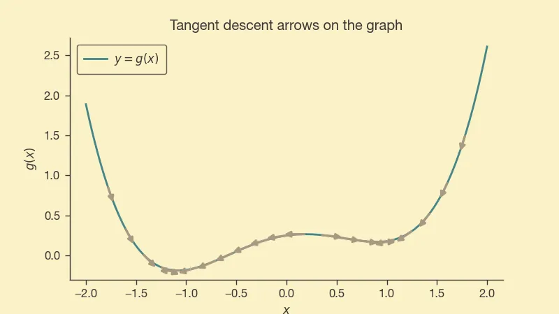
It behaves as we would expect, pointing trajectories towards the minima.

It would be fun to imagine various ways to lift the vector field from the curve $y = g (x)$ to $ℝ^{2}$ . There are infinite ways to do this.

First lift

We want to define a vector field $F : ℝ^{2} \to ℝ^{2}$ such that trajectories moving according to it converge to the minima¹ of $g$ .

To keep things simple, we will let $x^{'} = - g^{'} (x)$ . This way the horizontal axis behaves in the same way as if we are on the curve.

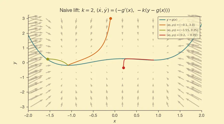
For the vertical axis, we will follow the idea of the previous post, i.e., $u = y - g (x)$ and we want $u^{'} = - k u$ for some $k > 0$ that we can pick. From this,

$u^{'} = y^{'} - g^{'} (x) x^{'} = - k u \Rightarrow y^{'} = g^{'} (x) x^{'} - k u .$

And so our differential equations are:

$x^{'} = - g^{'} (x)$

$y^{'} = g^{'} (x) x^{'} - k u .$

No matter how high $y_{0}$ is initially, the system will move towards the $g$ curve.

Here's how it looks like with $k = 2$ :

naive_lift

Second lift: have the dynamics of $y$ inform $x$ .

While the previous construction is simple, the $y$ axis movement is cosmetic, it is not playing any role in what we do on the $x$ axis (which is a waste and which is why we called it a “naive lift”).

As long as we pick $y^{'} = g^{'} (x) x^{'} - k u$ , we will still satisfy $u^{'} = - k u$ , i.e., exponential decay of $u$ , so we have some freedom in picking $x^{'}$ .

For example, we may want the dynamics of $x^{'}$ to ignore $g^{'}$ when $u$ is large enough, e.g., pick a $β > 0$ and set $x^{'} = - g (x) - β u$ . If $u$ is large, $x$ will move towards the left even if $g^{'}$ is pointing towards the right.

We went from

x^{'} = - g^{'} (x)

y^{'} = g^{'} (x) x^{'} - k u

x^{'} = - g^{'} (x) - β u

y^{'} = g^{'} (x) x^{'} - k u

This is what the dynamics look like in this case:

residual_lift

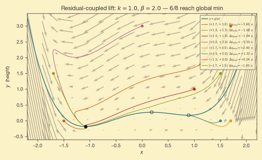
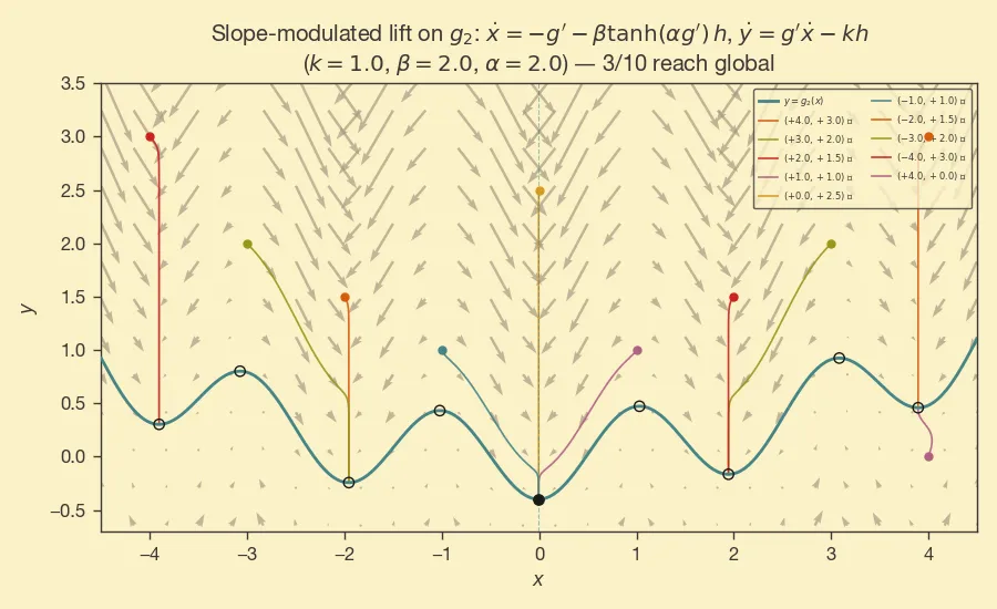
This is more interesting, but we are somewhat cheating -- the global min is to the left of the local min, and we have a method that is biased towards left movement. The behavior is clearer when the function is more complicated:

residual_lift_complex

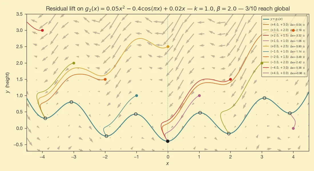
The further we are from $g$ , the more time the trajectory gets to skip a few of the basins as it moves towards the left.

Third lift

We have the freedom to pick the ODE for $x^{'}$ and get the same exponential convergence of the residual $u^{'} = - k u$ . That is, for any $B : ℝ^{2} \to ℝ$ , we are free to define the ODE of $x^{'}$ as

$x^{'} = - g^{'} (x) + B (x, y) u$

We can get a few different behaviors by playing with $B$ . For example:

slope_modulated_lift

To sum up, we looked at trajectories off of $g$ that converge to minima of $g$ . There's freedom in picking the form of the ODE of $x^{'}$ , so we can get different dynamics, avoidance, etc.

Technically stationary points.↩

Lifting gradient flows

First lift

Second lift: have the dynamics of y inform x.

Third lift

Second lift: have the dynamics of $y$ inform $x$ .