Greedy Coordinate Gradient

25 Feb, 2026

TL;DR: My notes on the “Greedy Coordinate Gradient”, first read from Zou, et al, 2023¹, but slightly abstracted.

Suppose we have the set $\Sigma =\{1,\dots ,N\}$, a function from sequences of $n$ elements to a vector space: $f:{\Sigma }^n\to {ℝ}^{n\times d}$, and another one $g:{ℝ}^{n\times d}\to {ℝ}^{\ge 0}$, $g$: differentiable. We want to minimize $L(x)=g(f(x))$ where $x\in {\Sigma }^n$.

First approach: Try all combinations $x\in {\Sigma }^n$ till we find the one that minimizes $L(x)$. Not very promising, too many trials.

Second approach: We would love to use gradients to guide the search, but we can’t — $\Sigma$ is a discrete set! However, nobody said we cannot take a gradient of $g$ with respect to $f:{\nabla }_{f}g.$ So an algorithm idea goes as follows: we start with $x_0\in {\Sigma }^n$ and then compute $y_0=f(x_0)$.

From here, $v_0=-{\nabla }_{y}g(y){|}_{y=y_0}$ gives us the direction to move towards (this is an $n\times d$ matrix), but there is a problem — the optimal direction may not be available! After all we only have the $V=\{f(x):x\in {\Sigma }^n\}$ points to work with. So, to make do with what we have, we can find the direction that is most aligned with where the gradient wants to go, i.e.,

(although using cosine similarity may be a better idea -- the idea of solving the linear problem is from Frank and Wolfe²).

And if we arrange the elements of $V$ in a matrix $A$, we can then $A{u}_0$ to compute all similarities at once.

Now we can iteratively update the elements of a sequence $x\in {\Sigma }^n$ by computing $\lambda (x^{\prime })$, where $x’$ is equal to $x$ in all positions except one, i.e., we consider all single-element swaps with elements from $\Sigma$ (there are $O(n·N)$ such sequences in total if we only do single element swaps). However, we can consider the top-k best $\lambda (x’)$ and then compute $G(x’)$ for each one of them and select the one with the smallest $G$. Then we repeat.

Code

Here’s a practical example with a convex loss and the minimum at $(0,0)$ (if we are only optimizing $g(f)$ instead of $g(f(x))$). To keep things simple, we will assume $d=1$ and $n=2$, but this is without losing any of the generality. ³

import mlx.core as mlxc

VOCAB_SIZE = 10000
D = 4
CRITICAL = 0

vocab = list(range(VOCAB_SIZE))
embd = mlxc.random.normal([VOCAB_SIZE, D])

def f(x: int | list[int]) -> mlxc.array:
    if isinstance(x, int) and x == CRITICAL: 
        return mlxc.zeros(D)
    
    if isinstance(x, list):
        elems = []
        for el in x: 
            if el == CRITICAL:
                elems.append(mlxc.zeros(D))
            else:
                elems.append(embd[el])
        return mlxc.stack(elems, axis=0)
    
    raise ValueError("Input must be an int or a list of ints")


def g(x: mlxc.array) -> mlxc.array:
    return mlxc.sum(x**2)

# function to minimize 
def G(x: int | list[int]) -> mlxc.array:
    return g(f(x))

grad_g = mlxc.grad(g)

seq = [0,10] # initial sequence 
SEQ_LEN = len(seq)
print("Initial sequence:", seq)
print("Initial loss:", G(seq))

NITER = 100 
TOPK = 10

best_loss = [G(seq)]
available_embds = embd[vocab]

for _ in range(NITER):
    grad = -grad_g(f(seq))
    candidates = []
    losses = []
    
    for i in range(SEQ_LEN):
        grad_i = grad[i]

		# scan the embedding matrix for promising swaps 
        similarities = mlxc.sum(grad_i * available_embds, axis=-1)
        similarities /= mlxc.linalg.norm(grad_i) * mlxc.linalg.norm(available_embds, axis=-1)
        topk_indices = mlxc.argsort(similarities)[-TOPK:]
 
        for idx in topk_indices:
            candidate = seq.copy()
            candidate[i] = int(idx)
            candidates.append(candidate)
            losses.append(float(G(candidate)))

    best_idx = min(range(len(losses)), key=lambda j: losses[j])

    seq = candidates[best_idx]
    best_loss.append(losses[best_idx])


import matplotlib.pyplot as plt
plt.plot(best_loss)
plt.xlabel("Iteration")
plt.ylabel("Best loss")
plt.title("Best loss over iterations")
plt.show()

print("Best sequence:", seq) 
print(f'Final loss: {best_loss[-1]}')

This does reduce the loss, though in typical coordinate-descent fashion it can get stuck. 😬

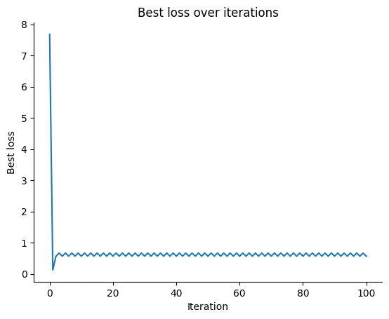
The trajectory depends on the available directions in $\{f(x):x\in {\Sigma }^n\}$. In the above plot, the algorithm stopped at [9998, 6304] with a final loss of 0.56.

To recap: We want to optimize $L$, but $L$ lives on a large finite space and we can’t use gradients directly. However, because of the decomposition $L(x)=g(f(x))$ we can use the gradient ${\nabla }_{f}g$ instead as a proxy, then do a linear scan to find the closest viable update within ${\Sigma }^n$.

Language models

For language models, $f$ is a map from token-sequence spaces to some hidden representation and $g$ maps the representation to the final loss value (as used in past works¹).

Someone may ask: what if we instead insert a new symbol in $\Sigma$ and extend $f$ so that $f(x)$ matches what the gradient expects? This then leads to methods like soft-prompting⁴ / prefix-tuning⁵.

Footnotes