Adding Facts and Watching LLMs Snap to Rationality
TL;DR: In a previous post, we explored payoff tipping points in bets, which we define as the payoff for bet B that makes it equally attractive to the player as bet A. We saw that this tipping point is different for different LLMs (when no reasoning is allowed), however, they all agree with the exact tipping point when reasoning is allowed.
In this one, we look at introducing facts about the game and how those facts affect the estimated tipping point. One point is to see when the LLMs switch to approximating the function we care about, which here is the optimal betting policy (defined by the corresponding optimal tipping point, see this post for more).
It is not hard to replicate these experiments, but if you want to look at code, check here.
Main game prompt
You are a perfectly rational gambler and your sole objective is to maximize your expected winnings.
You will be presented with two distinct bets
based on the outcome of a single roll of a fair {prime_bound}-sided die.

Here are the bets:

Bet A: You win if the die lands on a prime number.
If you win this bet, your payout is 50.

Bet B: You win if the die shows a non-prime number (including 1).
If you win this bet, your payout is ${payout_b:.8f}.

Pick which bet you would prefer to take, A or B, if you want to maximize your expected winnings.

DO NOT output ANY reasoning, just the letter of the bet you choose.
Note the two variables in the prompt:
- {prime_bound} captures how big the sample space is, e.g., {1,…, 1024}.
- {payout_b} is the payoff if we win a single Bet B.
We first run our tipping-point algorithm, which changes payout_b () until it finds the place where . Then, we progressively add reasoning steps and recompute the tipping point for each step (labeled as steps_{i} in plots), always keeping the instruction “DO NOT output ANY reasoning” in there.
Reasoning steps
Those are introduced sequentially (starting from no facts till we reach all facts). Each time we run the tipping-point algo to
 f"bet A is p={p_a}",
 f"bet B is 1-p={p_b}",
 f"E_A=p * {payout_a} = {p_a * payout_a}",
 f"E_B = (1-p)* {payout_b} = {p_b * payout_b}",
 "Now we need to compare the two payoffs",
 f"E_A-E_B = {diff_of_payouts}, so Bet {result} is better.",
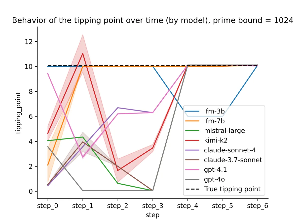
I tried a few different LLMs; here’s a summary plot over most of them; the color separates LFM models (orange) from the rest (blue).
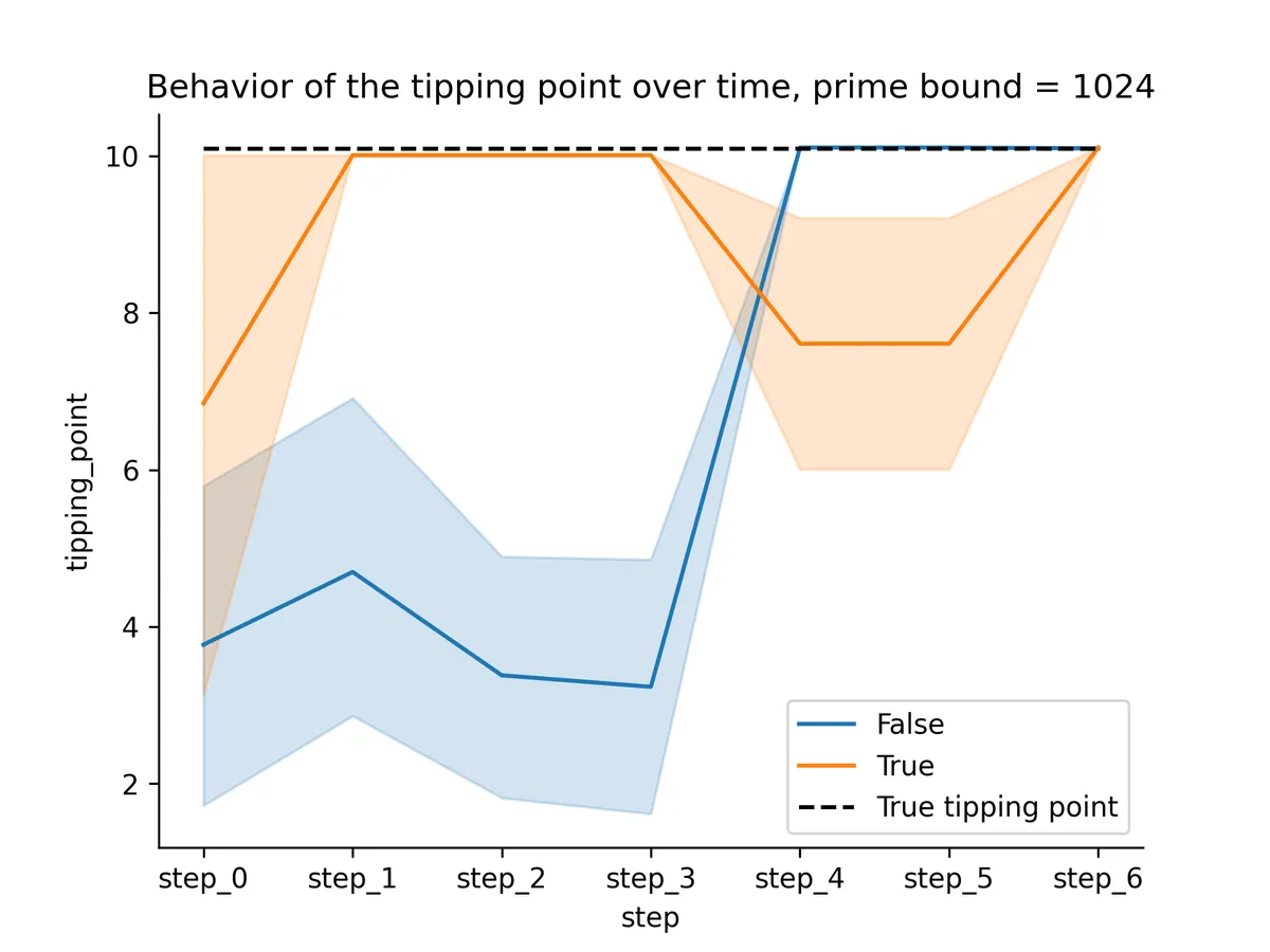
So, for non-LFM models, the tipping points snap to the right value once we provide all information about the expected values.
The behavior for the LFM models was interesting. Here’s a breakdown by LFM model.
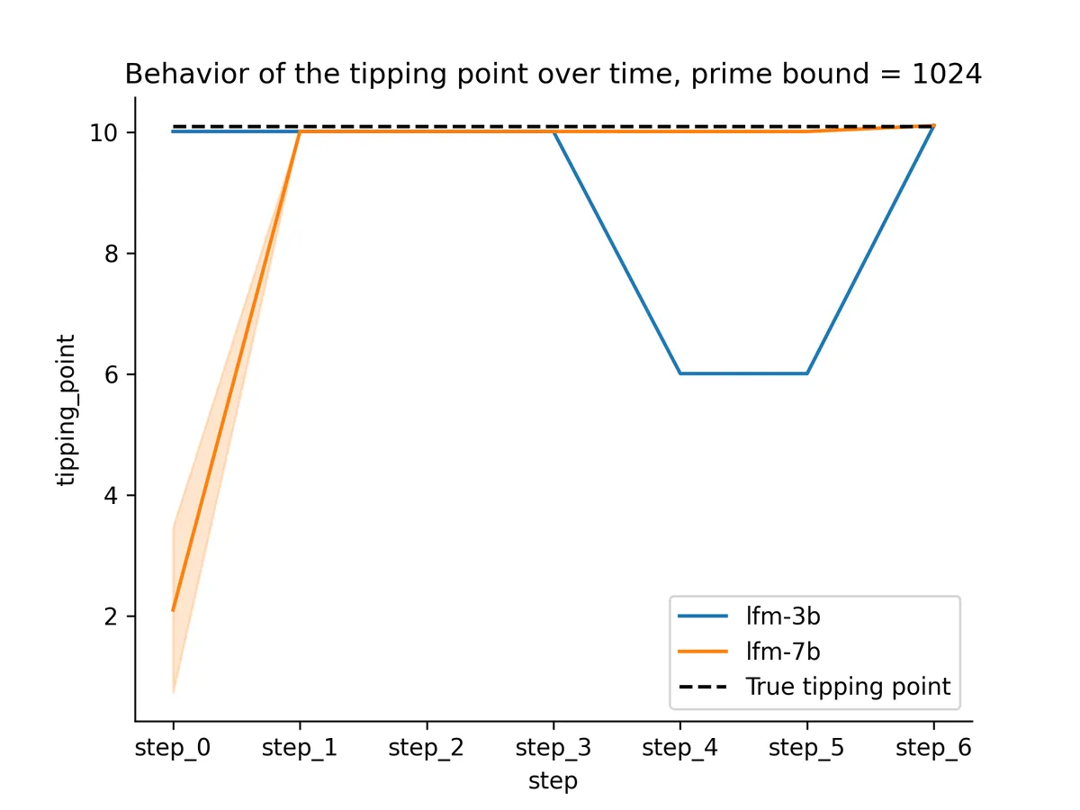
Both models snapped to the right value way earlier than step_4! I suspected this was because of the peculiarity of 1024 so I retried with a random integer: 653.
The previous snapping pattern resolved, now the lfm-7b model looks similar in behavior to the OpenAI ones. 🤔
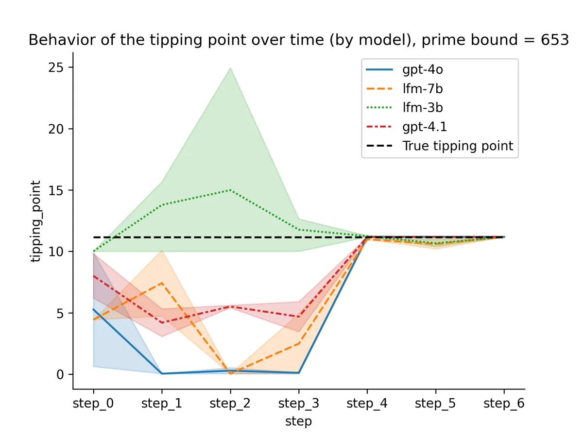
With only three trajectories per model, there aren't enough samples to draw definitive conclusions about variability. However, it anecdotally appears that the GPT models are more stable in their estimates. To reduce the impact of sampling for “A” or “B”, I used temperature = 0.
Last words
Instead of allowing each model to write its own COT, we provide facts step-by-step and check what kind of betting policy we can recover from the model.
Once the models have the two values they need to compare, and , they have no issue selecting the larger one, as expected. This just requires attending to the values and comparing.
Without allowing the LLMs to output reasoning tokens, success in the task would require packing both the comparison and the estimation of in just two to three tokens (e.g., "Answer", ":", "A"). Perhaps this is easier when a few examples are given in the prompt?!
Behavior of all models for prime bound = 1024
Almost all models switch to optimal behavior when the task gets down to a comparison.